Tutorial: Basics
Basic Concepts
QEpsilon is built around several key concepts:
Operators: Quantum operators in second-quantization formalism. Operators can be one-body operators or many-body operators.
Systems: Physical open quantum systems (many-body system consists of bosons, electrons, qubits, etc.) with a Hamiltonian, a set of Lindblad operators, and a set of parameters.
Simulations: Time evolution of quantum master equations.
A high-level overview of the architecture of QEpsilon is shown below:
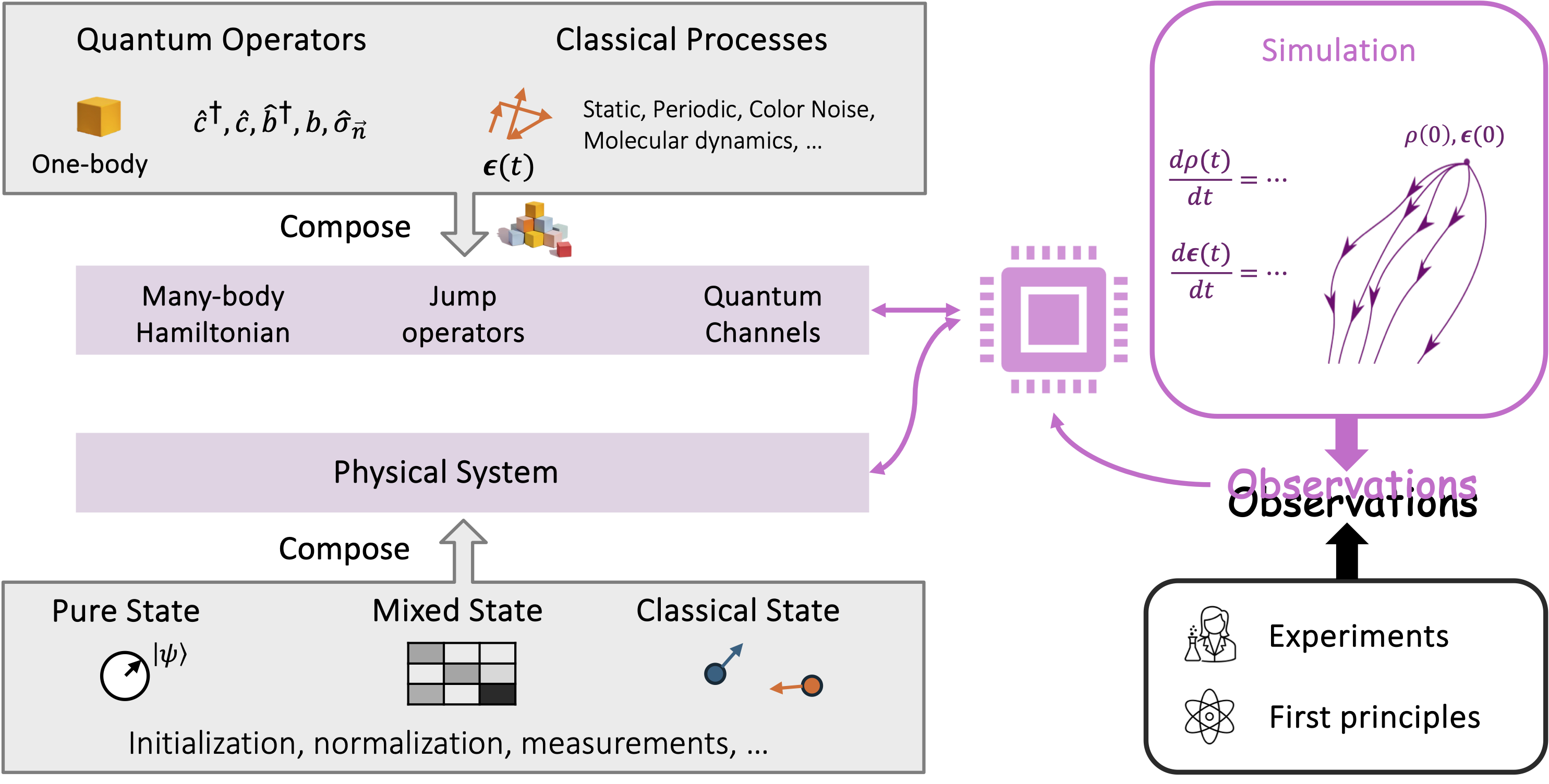
Architecture of QEpsilon
What is an operator in QEpsilon?
In QEpsilon, a Hamiltonian is a sum of OperatorGroups. Each OperatorGroup is a collection of many-body operators, acting on the same physical system, with a time-dependent coefficients. And each many-body operator is a tensor product of one-body base operators.
For example, a OperatorGroup can be a collection of many-body spin operators expressed in the Pauli basis. It can represent, for example, \(\epsilon(t) (a_1 \sigma^x_1 \otimes \sigma^x_2 + a_2 \sigma^y_1 \otimes \sigma^y_2)\). The scalar variable \(\epsilon(t)\) can be either static or time-dependent. The parameters within \(\epsilon(t)\) can be trained on data. Meanwhile, the scalar \(a_1\) and \(a_2\) are fixed prefactors of the operators. They can not be trained after initialization.
Alphabet of one-body base operators
There are currently three types of base operators underlying OperatorGroup: Pauli operators (e.g. \(\sigma^x, \sigma^y, \sigma^z\)), bosonic creation/annihilation operators (e.g. \(b^\dagger, b\)), and tight-binding hopping operators (e.g. \(c^\dagger_i c_j\)). We have an alphabet for each type of base operators, such that a one-body operator can be specified as a letter in the alphabet.
For spin systems, the alphabet is “I” (identity), “X” (Pauli-X), “Y” (Pauli-Y), “Z” (Pauli-Z), “U” (raising), “D” (lowering), “N” (number operator).
For bosonic systems, the alphabet is “U” (Creation, i.e. raising), “D” (Annhilation, i.e. lowering), “I” (identity), “N” (number operator).
For tight-binding systems, the alphabet is “X” (Do nothing), “L” (hopping to the left), “R” (hopping to the right), “N” (number operator).
These alphabets are defined in the operator_basis module.
With these alphabets, a many-body operator can be denoted as a string of letters in the alphabet. For example, we can denote the Pauli operator \(\sigma^x_1 \otimes \sigma^x_2\) as “XX”.
OperatorGroup: initialization
A OperatorGroup should be initialized with size of the many-body system, a unique identifer (ID), and a batchsize for sampling \(\epsilon(t)\). Then, the OperatorGroup can be equipped with a list of operators by calling OperatorGroup.add_operator with a string of letters in the alphabet.
Users do not always need to build a OperatorGroup from scratch. QEpsilon provides several pre-defined subclasses of OperatorGroup for typical physical systems, such as interacting two-level systems, quantum harmonic oscillators, and tight-binding chains.
Example: a spin OperatorGroup with static coefficient
The opetatorgroup \(\epsilon(t) (a_1 \sigma^x_1 \otimes \sigma^x_2 + a_2 \sigma^y_1 \otimes \sigma^y_2)\) can be initialized with a static coefficient that is a constant \(\epsilon(t)=2.0\):
operator_group = StaticPauliOperatorGroup(n_qubits=2, id="sigma_x_sigma_x", batchsize=1, coef=2.0, requires_grad = False)
operator_group.add_operator("XX", prefactor=1.0)
operator_group.add_operator("YY", prefactor=1.0)
StaticPauliOperatorGroup is a subclass of OperatorGroup. The operator \(a_1 \sigma^x_1 \otimes \sigma^x_2\) is added to the originaly empty OperatorGroup by calling add_operator with \(a_1=1.0\). The operator \(a_2 \sigma^y_1 \otimes \sigma^y_2\) is added to the originaly empty OperatorGroup by calling add_operator with \(a_2=1.0\).
requires_grad is a boolean flag to indicate whether the coefficient \(\epsilon(t)\) is a trainable parameter. If it is True, the coefficient can be optimized later, together with other parameters in the system. If it is False, the coefficient will be fixed.
add_operator can be called multiple times to add more operators to the OperatorGroup. The specification of the operators is a string of Pauli operator names by the convention of the Pauli operator basis. Obviously, “XX” means \(\sigma^x_1 \otimes \sigma^x_2\), “XY” means \(\sigma^x_1 \otimes \sigma^y_2\), etc.
Example: a spin OperatorGroup with time-dependent coefficient
One can also initialize a OperatorGroup with a time-dependent coefficient. For example, the Pauli opetator mentioned above can be initialized with a time-dependent coefficient \(\epsilon(t)\) that is a white noise:
operator_group = WhiteNoisePauliOperatorGroup(n_qubits=2, id="xx_noise", batchsize=1, amp=0.0001, requires_grad = True)
operator_group.add_operator("XX", prefactor=1.0)
operator_group.add_operator("YY", prefactor=1.0)
WhiteNoisePauliOperatorGroup is a subclass of OperatorGroup. The amp is the amplitude of the white noise. Because here we let requires_grad = True, the amplitude becomes a trainable parameter that can be optimized later, together with other parameters in the system.
Example: quantum harmonic oscillator
One can initialize a OperatorGroup for a quantum harmonic oscillator as \(H = \sum_{i=1}^{N_{max}} \omega (b^\dagger b + 1/2)\):
Note that we can not accomodate infinitely many energy levels in numerical simulations. Therefore, when working with bosonic modes, we always need to truncate the number of energy levels to a finite number \(N_{max}\).
operator_group = HarmonicOscillatorBosonOperatorGroup(num_modes=1, id="boson_harmonic", batchsize=1, nmax=10, omega = 1.0)
Advanced feature: Composite OperatorGroup for general systems
The two examples given above uses pre-defined subclass of OperatorGroup: StaticPauliOperatorGroup and WhiteNoisePauliOperatorGroup. Often, there are more complex operators that are not implemented in QEpsilon. For example, you may be dealing with a system with operator groups involving both spin and boson operators. For these general situations, you can create a Composite OperatorGroup by yourself. This is a powerful feature of QEpsilon that provides the flexibility to study many different open quantum systems. The Composite OperatorGroup is a subclass of OperatorGroup. It is initialized with a list of OperatorGroup. For example, a Composite OperatorGroup for a system with both spin and boson operators can be initialized as:
##
batchsize = 1
spin_boson_coupling = 1.0
nmax = 10

## spin_z is a one-body spin operator
spin_z = StaticPauliOperatorGroup(n_qubits=1, id="spinz", batchsize=batchsize, coef=1.0, requires_grad=False)
spin_z.add_operator('Z')

## boson_x is a boson operator (b^\dagger + b)
boson_x = StaticBosonOperatorGroup(num_modes=1, id="boson_x", nmax=10, batchsize=batchsize, coef= spin_boson_coupling, requires_grad=False)   # gw(b^\dagger + b)
boson_x.add_operator('U')
boson_x.add_operator('D')

spin_boson_coupling = ComposedOperatorGroups(id="spin_boson_couple", OP_list=[spin_z, boson_x])
Here, we first define a spin-z operator \(\sigma^z\) and a boson operator \(b^\dagger + b\). Then, we compose them into Composite OperatorGroup with the ID “spin_boson_couple” and the expression \(\sigma^z \otimes (b^\dagger + b)\).
How to define a quantum/classical state?
Because QEpsilon is made for mixed quantum classical simulations. It implements multiple type of states of a physical system:
Density matrix: the density matrix of a mixed or pure quantum state.
Pure quantum state: the wavefunction of a pure quantum state.
Classical particles: the positions and momenta of classical particles.
These states are implemented in the system module.
Density matrix
The parent class of density matrix is DensityMatrix. It is initialized with the number of states and the batchsize. For example, a density matrix of a two-level qubit system can be initialized as:
import torch as th
from qepsilon import DensityMatrix
density_matrix = DensityMatrix(num_states=2, batchsize=1)
rho = th.tensor([[1.0, 0.0], [0.0, 1.0]], dtype=th.cfloat)
density_matrix.set_rho(rho)
The density matrix is a complex tensor of shape (batchsize, num_states, num_states). DensityMatrix does not restrict the type of the underlying physical system, which can be spin-like, bosonic, or mixed-type. Essentially, it is just a wrapper of a complex tensor.
DensityMatrix has a setter function set_rho to set the density matrix, and a getter function get_rho to get the density matrix. DensityMatrix has a property trace to get the trace of the density matrix. DensityMatrix has a method normalize to normalize a given density matrix (it does not update the stored density matrix automatically).
Subclass of DensityMatrix
A subclass of DensityMatrix is QubitDensityMatrix. It is initialized with the number of qubits and the batchsize. It is used to represent the density matrix of a finite number of 2-level qubits. It has a few dedicated methods such as set_rho_by_config to set the density matrix by a configuration vector, partial_trace to perform a partial trace with respect to a subset of qubits, apply_unitary_rotation to apply a unitary rotation on a selected subset of qubits, and observe_paulix_one_qubit to observe the Pauli-X operator of one qubit.
Pure quantum state
The parent class of pure quantum state is PureStatesEnsemble. It is initialized with the number of states and the batchsize. For example, a pure state ensemble of a two-level qubit system can be initialized as:
from qepsilon import PureStatesEnsemble
pure_states_ensemble = PureStatesEnsemble(num_states=2, batchsize=1)
pse = th.tensor([1.0, 0.0], dtype=th.cfloat)
pure_states_ensemble.set_pse(pse)
The pure states ensemble is a complex tensor of shape (batchsize, num_states). PureStatesEnsemble has a setter function set_pse to set the pure states ensemble, and a getter function get_pse to get the pure states ensemble. PureStatesEnsemble has a method normalize to normalize a given pure states ensemble (it does not update the stored pure states ensemble automatically). PureStatesEnsemble has a method get_expectation to get the expectation of an operator (a plain square matrix, not an OperatorGroup) on the pure states ensemble.
Subclass of PureStatesEnsemble
So far, there are two subclasses of PureStatesEnsemble: TightBindingPureStatesEnsemble and QubitPureStatesEnsemble.
They are used to represent the pure states ensemble of tight-binding systems and qubit systems, with a few dedicated methods for convenience.
Classical particles
The parent class of classical particles is Particles. It is initialized with the number of particles, the batchsize, the dimension of the space, the mass of the particles, and optionally also the time step for their dynamical evolution. For example, a classical particles system of two particles in 3D space can be initialized as:
from qepsilon import Particles
particles = Particles(n_particles=2, batchsize=1, ndim=3, mass=1.0, dt=0.1)
positions = th.tensor([[0.0, 0.0, 0.0], [1.0, 1.0, 1.0]], dtype=th.float32)
particles.set_positions(positions)
particles.set_gaussian_velocities(temp=300.0)  ## default temperature unit is Kelvin
Particles has a setter function set_positions to set the positions of the particles, and a setter function set_gaussian_velocities to set the velocities of the particles as a Gaussian distribution. Particles has a getter function get_positions to get the positions of the particles, and a getter function get_velocities to get the velocities of the particles. Particles has a method modify_forces to modify the forces on the particles.
Classical Molecular Dynamics of Particles
Particles has a method step_langevin to perform a Langevin dynamics step.
It updates the positions and velocities of the particles by one time step with force, damping, and white noise.
The force is stored as particles.forces. It can be reset to zero by calling particles.zero_forces().
And it can be modified by calling particles.modify_forces.
Particles has a method step_adiabatic to perform an adiabatic dynamics step.
It updates the positions and velocities of the particles by one time step with leapfrog method, using the force stored in particles.forces.
Next Steps
See the Tutorial: Simulation for how to simulate a physical system with the components defined in this section