Tutorial: Training
Introduction
This tutorial demonstrates how to train a data-informed quantum-classical dynamics (DIQCD) model using QEpsilon. QEpsilon provides a simulation-based method to train the parameters of a quantum system from experimental or simulation data.
Basically, the training process involves the following steps:
Define the physical system (Hamiltonian, jumping operators, etc.) like how you define the system in the Tutorial: Simulation section. But remember to specify that requires_grad=True for those operators that are to be trained. Keep requires_grad=False for those operators that are known a priori.
Simulate the system dynamics like how your (actual or numerical) experiments are performed. Make measurements at those time steps that you have data for.
Calculate the loss function between the simulated data and the experimental data. You can use any metric you like. For example, you can use the mean squared error (MSE) between the simulated data and the experimental data.
Do a standard optimization procedure to minimize the loss function.
Example: Two-level system
Here we demonstrate how to train a DIQCD model for a one-qubit system, with data from a Ramsey experiment.
The Ramsey experiment is a standard experiment to measure the coherence time of a qubit. The Ramsey experiment is performed by applying a pi/2 rotation along the x-axis, then free evolution for a time \(t\), and then applying a pi/2 rotation along another axis (flexible, denoted by \(u\) in the following).
The observation is performed by measuring the probability of being in the state \(|0\rangle\) (spin-up) at the end of the experiment. Let this probability be denoted by \(P_{\uparrow}(t,\theta)\).
Let \(u=(cos(\theta), sin(\theta), 0)\). We define the Ramsey contrast as \(C(t) = |P_{\uparrow}(t,\theta=\pi) - P_{\uparrow}(t,\theta=0)|\).
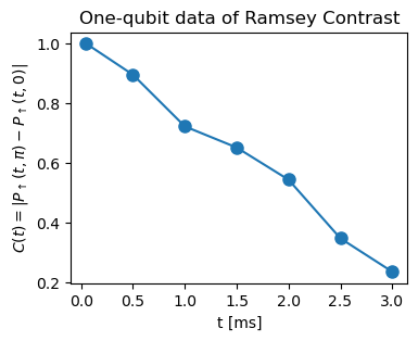
Below is a set of data of Ramsey contrasts extracted from Holland et al., Science 382, 1143–1147 (2023). The Ramsey contrasts are preprocessed to eliminate preperation errors.
## a simple time series data of Ramsey experiments. Ramsey contrasts are measured for T=0.05ms, 0.5ms, 1.0ms, 1.5ms, 2.0ms, 2.5ms, 3.0ms
measure_t = [0.0500, 0.5000, 1.0000, 1.5000, 2.0000, 2.5000, 3.0000]
measure_C = [1.0000, 0.8958, 0.7227, 0.6518, 0.5439, 0.3473, 0.2354]
fig, ax = plt.subplots(figsize=(4,3))
ax.plot(measure_t, measure_C, markersize=8, marker='o')
ax.set_xlabel('t [ms]')
ax.set_ylabel(r'$C(t)=|P_{\uparrow}(t,\pi) - P_{\uparrow}(t,0)|$')
ax.set_title('One-qubit data of Ramsey Contrast')
plt.show()
plt.close()
Let us then establish a DIQCD model to fit the data.
import numpy as np
import torch as th
import qepsilon as qe
from matplotlib import pyplot as plt
batchsize = 256
qubit = qe.QubitLindbladSystem(n_qubits=1, batchsize=batchsize)
qubit.set_rho_by_config([0])
sz_shot = qe.ShotbyShotNoisePauliOperatorGroup(n_qubits=1, id="sz_noise_shot", batchsize=batchsize, amp=0.1, requires_grad=True)
sz_shot.add_operator('Z')
qubit.add_operator_group_to_hamiltonian(sz_shot)

sx_jump = qe.StaticPauliOperatorGroup(n_qubits=1, id="sx_jump", batchsize=batchsize, coef=0.01, static=False,requires_grad=True)
sx_jump.add_operator('X')
qubit.add_operator_group_to_jumping(sx_jump)
Up to this point, what we do is almost the same as how we define the qubit Lindblad system in the Tutorial: Simulation section. The only difference is that we set requires_grad=True for both Hamiltonian and jumping operators.
Next, we set the simulation and training parameters.
dt=0.005 ## time step
T=4 ## total simulation time
nsteps = int(T/dt)
observe_steps = [int(t / dt) for t in measure_t]  ## do measurement at these time steps
nepoch = 100  ## total training epoches
optimizer = th.optim.Adam([{'params': qubit.HamiltonianParameters(), 'lr': 0.03},
                          {'params': qubit.JumpingParameters(), 'lr': 0.001}])
The meaning of these parameters are self-explanatory. At the end, we set a ADAM optimizer for the parameters in the DIQCD model. HamiltonianParameters() is the set of all the trainable parameters in the Hamiltonian, and JumpingParameters() is the set of all the trainable parameters in the jumping operators.
Now, we are ready to perform simulation, compare with the data, and train the model, in an iterative manner.
for epoch in range(nepoch):
    ## reset system state
    qubit.reset()
    qubit.set_rho_by_config([0])
    prob_up_list = []  ## for storing the measurement results

    # apply first pi/2 rotation along x
    qubit.rotate(direction=th.tensor([1.0,0,0]), angle=np.pi/2)

    # free evolution and measurement
    for i in range(nsteps):
        qubit.step(dt=dt)
        if i in observe_steps:
            for theta in [0, np.pi]:
                # define the axis for applying the last pulse
                u = th.tensor([np.cos(theta), np.sin(theta), 0.0], dtype=th.float)
                # apply the second pi/2 rotation along the direction u
                dm = qubit.density_matrix
                current_rho = dm.apply_unitary_rotation(qubit.rho, u, np.pi/2)
                # observe the probability of being in the state |0>  (spin-up)
                prob_up = dm.observe_prob_by_config(current_rho, th.tensor([0]))
                prob_up_list.append(prob_up.mean())

    ## calculate loss and step optimizer
    prob_up_list = th.stack(prob_up_list).reshape(len(observe_steps), 2)
    Ramsey_Contrast = th.abs(prob_up_list[:, 1] - prob_up_list[:, 0])
    loss = ((Ramsey_Contrast - th.tensor(measure_C)) ** 2).mean()
    optimizer.zero_grad()
    loss.backward()
    optimizer.step()

    if epoch % 10 == 0:
        print('Epoch={}, Loss={}'.format(epoch, loss))
        print('Simulated Ramsey Contrast:', Ramsey_Contrast.detach().numpy())
The training quickly converges to a good fit. Output is shown below.
Epoch=0, Loss=0.13371221721172333
Simulated Ramsey Contrast: [0.9999263  0.9945936  0.97892886 0.9534482  0.91886765 0.8761416
 0.8264214 ]
Epoch=10, Loss=0.10416834056377411
Simulated Ramsey Contrast: [0.999856   0.9912077  0.96643484 0.9270018  0.87496626 0.81293535
 0.7438406 ]
Epoch=20, Loss=0.03927537053823471
Simulated Ramsey Contrast: [0.9996637  0.97956324 0.9235978  0.83931565 0.7365615  0.6254713
 0.51449037]
Epoch=30, Loss=0.011041725054383278
Simulated Ramsey Contrast: [0.9994703  0.9691173  0.8858475  0.7633902  0.6198219  0.47379768
 0.3406668 ]
Epoch=40, Loss=0.005107288248836994
Simulated Ramsey Contrast: [0.9991515  0.94778126 0.81110644 0.6247592  0.4319702  0.26973945
 0.15821564]
Epoch=50, Loss=0.006070218048989773
Simulated Ramsey Contrast: [0.99913985 0.94839346 0.8131318  0.626911   0.43046987 0.2592173
 0.13389939]
Epoch=60, Loss=0.0035872850567102432
Simulated Ramsey Contrast: [0.9992665  0.9583786  0.84986055 0.6995914  0.53755385 0.38852668
 0.26703283]
Epoch=70, Loss=0.0028746577445417643
Simulated Ramsey Contrast: [0.99916273 0.9496452  0.819366   0.6445786  0.46642804 0.31605113
 0.2062841 ]
Epoch=80, Loss=0.0030608363449573517
Simulated Ramsey Contrast: [0.9991818  0.95154196 0.8250345  0.65181637 0.47051635 0.31374782
 0.19886565]
Epoch=90, Loss=0.003072070423513651
Simulated Ramsey Contrast: [0.9992282  0.9563436  0.8414374  0.6795628  0.50178504 0.3365388
 0.2025435 ]
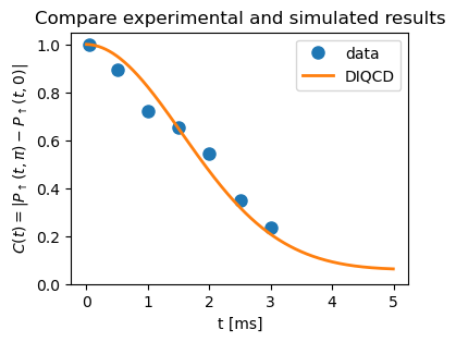
We are done. Below, we do a final simulation, with dense sampling of \(t\), to compare the simulated results with the experimental data.
qubit.reset()
qubit.set_rho_by_config([0])
prob_up_list = []  ## for storing the measurement results
nsteps = int(5/dt)
with th.no_grad():
    # apply first pi/2 rotation along x
    qubit.rotate(direction=th.tensor([1.0,0,0]), angle=np.pi/2)
    # free evolution and measurement
    for i in range(nsteps):
        qubit.step(dt=dt)
        for theta in [0, np.pi]:
            # define the axis for applying the last pulse
            u = th.tensor([np.cos(theta), np.sin(theta), 0.0], dtype=th.float)
            # apply the second pi/2 rotation along the direction u
            dm = qubit.density_matrix
            current_rho = dm.apply_unitary_rotation(qubit.rho, u, np.pi/2)
            # observe the probability of being in the state |0>  (spin-up)
            prob_up = dm.observe_prob_by_config(current_rho, th.tensor([0]))
            prob_up_list.append(prob_up.mean())

prob_up_list = th.stack(prob_up_list).reshape(-1, 2)
Ramsey_Contrast = th.abs(prob_up_list[:, 1] - prob_up_list[:, 0])
fig, ax = plt.subplots(figsize=(4,3))
ax.plot(measure_t, measure_C, markersize=8, marker='o', linewidth=0, label='data')
ax.plot(np.arange(Ramsey_Contrast.shape[0])*dt, Ramsey_Contrast.numpy(), linewidth=2, label='DIQCD')
ax.set_ylim(0, 1.05)

ax.set_xlabel('t [ms]')
ax.set_ylabel(r'$C(t)=|P_{\uparrow}(t,\pi) - P_{\uparrow}(t,0)|$')
ax.set_title('Compare experimental and simulated results')
ax.legend()
plt.show()
plt.close()
Next Steps
Explore the Examples sections for advanced examples
Check the API Reference for complete API reference